VASP workflow

VASP workflow demo.

# Import VASP calculator and unit modules
from ase.calculators.vasp import Vasp
from ase import units as un
from os.path import isfile
import os

# The sample generator, monitoring display and dfset writer
from hecss import HECSS
from hecss.util import write_dfset
from hecss.monitor import plot_stats

# Numerical and plotting routines
import numpy as np
from matplotlib import pyplot as plt
from collections import defaultdict
from tempfile import TemporaryDirectory
from glob import glob

# Quick test using conventional unit cell
supercell = '1x1x1'

# Slow more realistic test
supercell = '2x2x2'

# Directory in which our project resides
base_dir = f'example/VASP_3C-SiC/{supercell}/'
calc_dir = TemporaryDirectory(dir='TMP')

# Read the structure (previously calculated unit(super) cell)
# The command argument is specific to the cluster setup
calc = Vasp(label='cryst', directory=f'{base_dir}/sc_{supercell}/', restart=True)

# This just makes a copy of atoms object
# Do not generate supercell here - your atom ordering will be wrong!
cryst = calc.atoms.repeat(1)

# Setup the calculator - single point energy calculation
# The details will change here from case to case
# We are using run-vasp from the current directory!
calc.set(directory=f'{calc_dir.name}/sc')
calc.set(command=f'{os.getcwd()}/run-calc.sh "vasp_test"')
calc.set(nsw=0)
cryst.set_calculator(calc)

print('Stress tensor: ', end='')
for ss in calc.get_stress()/un.GPa:
    print(f'{ss:.3f}', end=' ')
print('GPa')

Stress tensor: 0.017 0.017 0.017 0.000 0.000 0.000 GPa

# Prepare space for the results.
# We use defaultdict to automatically
# initialize the items to empty list.
samples = defaultdict(lambda : [])

# Space for amplitude correction data
xsl = []

# Build the sampler
hecss = HECSS(cryst, calc, 
              directory=calc_dir.name,
              w_search = True,
              pbar=True,
              )

N = 5
m, s, xscl = hecss.estimate_width_scale(5, nwork=0)
wm = np.array(hecss._eta_list).T
y = np.sqrt((3*wm[1]*un.kB)/(2*wm[2]))
plt.plot(wm[1], y, '.');
x = np.linspace(0, 1.05*wm[1].max(), 2)
fit = np.polyfit(wm[1], y, 1)
plt.plot(x, np.polyval(fit, x), ':', label=f'{fit[1]:.4g} {fit[0]:+.4g} T')
plt.axhline(m, ls='--', label=f'{m:.4g}±{s:.4g}')
plt.axhspan(m-s, m+s, alpha=0.3)
plt.ylim(m-4*s, m+4*s)
plt.xlabel('Target temperature (K)')
plt.ylabel('width scale ($\\AA/\\sqrt{K}$)')
plt.legend();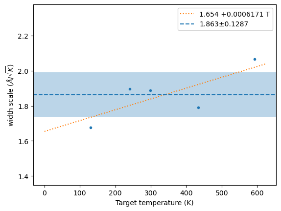

# Desired number of samples and T list.
N = 30
T_list = (100, 200, 300)
for T in T_list:
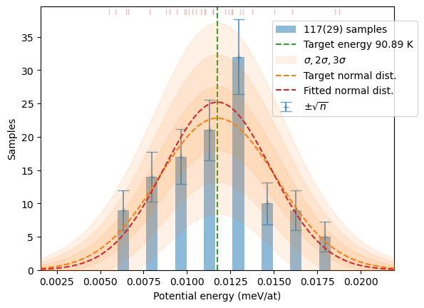
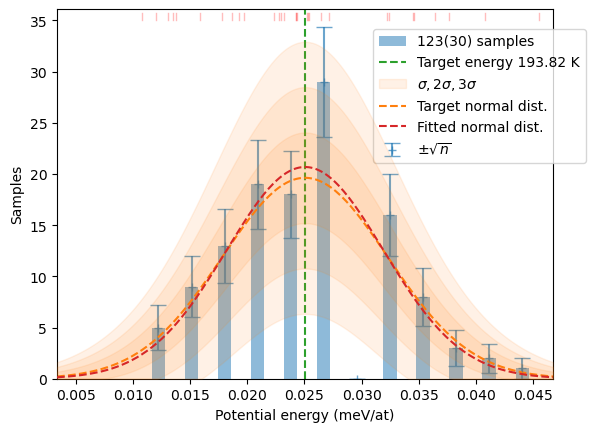
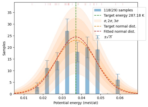
    samples[T] += hecss.sample(T, N)

# Plot the resulting distributions
for T in T_list:
    plot_stats(hecss.generate(samples[T]), sqrN=True)