Post-processing procedure to match the sampling set to the target distribution by adjusting the data weights in the sample.
This code is an implementation of the idea to replace crude weighting produced by the Metropolis-Hastings algorithm by weights derived directly from the PDF of the target distribution. This makes the acceptance ratio essentially 100% and allows for tricks like changing of the target distribution (e.g. shifting of the target temperature of the sample or even scanning of the temperature range using prior distribution generated using plan_T_scan).
The implementation here, derives the weights directly from the PDF of the target distribution by assigning non-uniform bins to each data point and calculating change in CDF across each bin. The resulting data uses weighting in similar way as the M-H sampling does, but exploits the knowledge of the sample distribution and target PDF to make it more effective.
*Generate data weights making the probability distribution of data in sample format into normal distribution corresponding to temperature T. The actual distribution traces the normal curve. Normally, no weight is given to the data outside the input data range. This may skew the resulting distribution and shift its parameters but avoids nasty border artefacts in the form of large weights given to border samples to account for the rest of the domain. You can switch this behavior on by passing border parameter (not recommended).
Input
data - list of samples generated by HECSS sampler ([n, i, x, f, e])
T - temperature in kelvin
sigma_scale - scaling factor for variance. Defaults to 1.0.
border - make border samples account for unrepresented part of domain
debug - plot diagnostic plots
Output (weights, index)
weights - array of weights in sorted energy order
index - indexing array which sorts samples by energy*
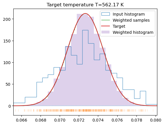
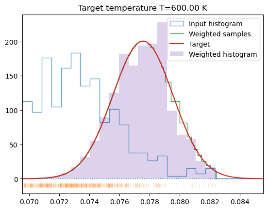
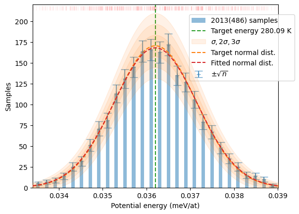
# Calculate the mean of the sample# We do not care too much about which temperature we got# Just if we are in equilibriumTmu = np.fromiter((s[-1] for s in smpls), float).mean()Tmu *=2/un.kB/3# Get weights for this temperatureplt.title(f'Target temperature T={Tmu:.2f} K')wgh, idx = get_sample_weights(smpls, Tmu, border=False, debug=True)# and now for actual target temperature Tplt.title(f'Target temperature T={T:.2f} K')wgh, idx = get_sample_weights(smpls, T, border=False, debug=True)
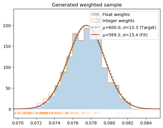
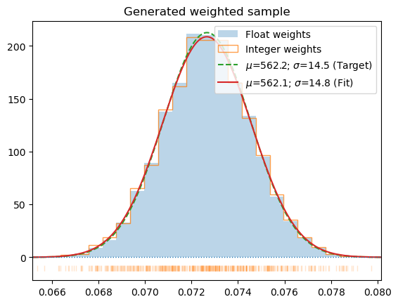
*Generate new sample with normal energy probability distribution corresponding to temperature T and size of the system inferred from data. The output is generated by multiplying samples proportionally to the wegihts generated by get_sample_weights and assuming the final dataset will be Nmul times longer (or the length N which takes precedence). If nonzero_w is True the data multiplyers in the range (probTH, 1) will be clamped to 1, to avoid losing low-probability data. This will obviously deform the distribution but may be beneficial for the interaction model constructed from the data. The data on output will be ordered in increasing energy and re-numbered. The configuration index is retained.
Input
data - list of samples generated by HECSS sampler ([n, i, x, f, e])
T - temperature in kelvin
sigma_scale - scaling factor for variance. Defaults to 1.0.
border - make border samples account for unrepresented part of domain
probTH - threshold for probability (N*weight) clamping.
Nmul - data multiplication factor. The lenght of output data will be approximately Nmul*len(data).
N - approximate output data length. Takes precedence over Nmul
nonzero_w - prevent zero weights for data with weights in (probTH, 1) range
debug - plot diagnostic plots
Output
Weighted, sorted by energy and re-numbered samples as a new list. The data in the list is just reference-duplicated, not copied. Thus the data elements should not be modified. The format is the same as the data produced by HECSS sampler.*
Target temperature control
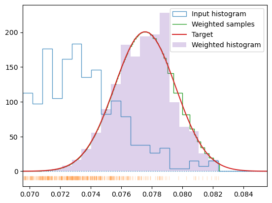
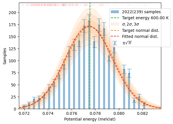
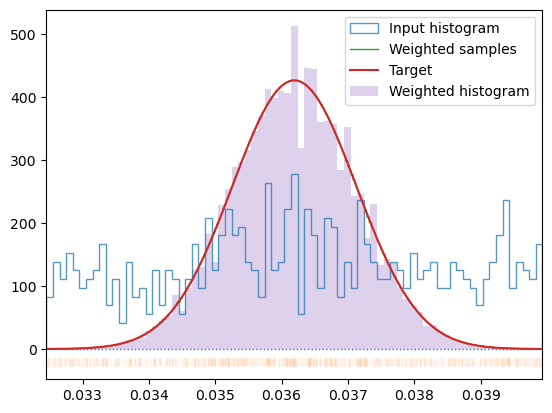
If the amplitude of displacement is not tightly controlled by the width searching algorithm (w_search parameter in the HECSS constructor), the mean energy of the sample will be shifted from the target value. The distribution reshaping algorithm in make_sampling may shift the result closer to the target but cannot create data out of thin air. This is illustrated in the example below. In first case (Section 1.1) we have forced the algorithm to create distribution at initial target temperature (T), which produces very distorted sample.
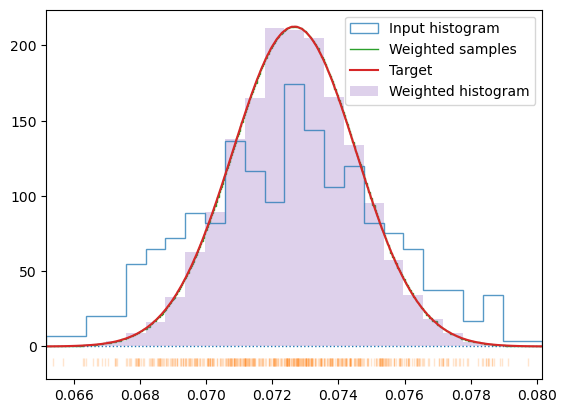
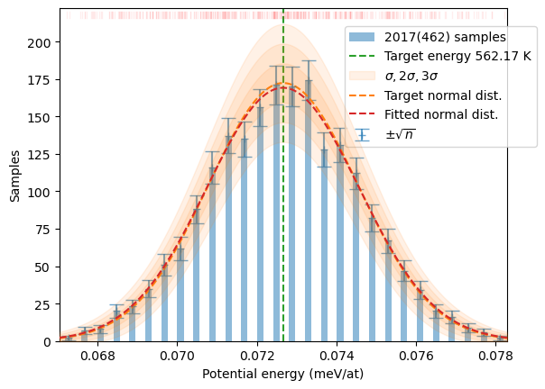
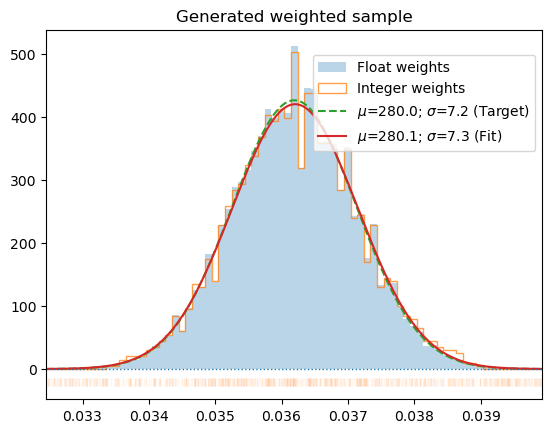
In the second case (Section 1.2) the target temperature is selected well within the data domain (Tmu which is actually the mean of the sample) which generates a well-balanced and uniform sampling of the target distribution, although at a slightly shifted temperature.
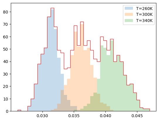
The ability to re-shape the sample makes it possible to scan the whole range of temperatures by adding samples from several temperatures and subsequently drawing from the whole set samples representing any target temperature in the covered range. The sampled temperatures may be selected manually or using automatic procedure from plan_T_scan. Here we just select few temperatures and run the procedure to test the weighting procedure on the non-gaussian prior.
uni = {TT:hecss.sample(TT, N) for TT in (260, 300, 340)}
e_dist = {t:np.array([s[-1] for s in d]) for t, d in uni.items()}e_uni = np.concatenate(tuple(e_dist.values()))usmp = []for s in uni.values(): usmp += sfor TT, ed in e_dist.items(): plt.hist(ed, bins=40, label=f'T={TT}K', alpha=0.25, range=(e_uni.min(), e_uni.max()))plt.hist(e_uni, bins=40, histtype='step', stacked=True, range=(e_uni.min(), e_uni.max()))plt.legend();