CLI

The command line interface for the HECSS sampler

Command line hecss sampler

The HECSS sampler can be also used from the command line using hecss-sampler command:

$ hecss-sampler -V

HECSS, version 0.5.15
High Efficiency Configuration Space Sampler
(C) 2021-2022 by Paweł T. Jochym
    License: GPL v3 or later

$ hecss-sampler --help

Usage: hecss-sampler [OPTIONS] FNAME

  Run HECSS sampler on the structure in the provided file (FNAME) Read the
  docs at: https://jochym.github.io/hecss/

  FNAME - Supercell structure file. The containing 
          directory must be readable by Vasp(restart).
          Usually this is a CONTCAR file for a supercell.

Options:
  -W, --workdir PATH      Work directory
  -l, --label TEXT        Label for the calculations.
  -T, --temp FLOAT        Target temperature in Kelvin.
  -w, --width FLOAT       Initial scale of the prior distribution
  -a, --ampl PATH         Initialise amplitude correction from the file.
  -s, --scale PATH        Save amplitude correction history
  -m, --symprec FLOAT     Symmetry search tolerance.
  -C, --calc TEXT         ASE calculator to be used for the job. Supported
                          calculators: VASP (default)
  -n, --nodfset           Do not write DFSET file for ALAMODE
  -d, --dfset TEXT        Name of the DFSET file
  -N, --nsamples INTEGER  Number of samples to be generated
  -e, --neta INTEGER      Number of samples for width scale estimation
  -c, --command TEXT      Command to run calculator
  -k, --nwork INTEGER     Number of parallel workers to run (0=unlimited)
  -p, --pbar              Do not show progress bar
  -V, --version           Show the version and exit.
  -h, --help              Show this message and exit.

To use it you need to prepare:

run-calc script which should start the VASP calculation. You need to put this script in the root of your project tree. The example of such a script is included in the source as run-calc.example. :

#!/bin/bash

# This script should run vasp in current directory 
# and wait for the run to finish.
# 
# A generic line using SLURM would look like this:
#
# sbatch [job_params] -W vasp_running_script
#
# The "-W" param makes the sbatch command wait for the job to finish.


JN=`pwd`
JN=`basename ${JN}`

# Partition of the cluster
PART=small

# Number of nodes
N=1

# Number of MPI tasks
ntask=64

# Name the job after directory if no label is passed as first argument
if [ "${1}." != "." ]; then
  JN=${1}
fi

sbatch -W -J ${JN} -p $PART -N $N -n $ntask run-vasp-script

A directory with fully converged and optimized supercell structure which can be read in by the ASE Vasp(restart=...) command
A directory for the generated samples.

The directory tree may look like this:

my_project ----- sc
             |
             +-- T_100
             |
             +-- T_200
             |
             +-- ...
             |
             +-- run-calc

You execute the sampler from the my_project directory (remember to activate your virtual environment first). Generation of N=30 samples at T=100K:

~$ cd my_project
~$ hecss_sampler -W T_100 -T 100 -N 30 -c ./run-calc sc/CONTCAR

The above command will put the generated samples inside the T_100 directory, together with the DFSET file with displacement-force data extracted from the calculation. The calculation may take a long time. Thus it is advisable to execute the hecss command inside screen (or some similar terminal multiplexer) to prevent the break of the calculation in case of session disconnection. The hecss command shows a progress to guide you through the calculation (ETA, time/it, data about last sample etc.). The example run is included at the bottom of this document.

Width scale estimation

Calling the sampler with N=0 runs only width scale (eta) estimation procedure for the temperature range 0-T Kelvin. The calculated value may be used as the -w parameter in subsequent calculations. Possibly even for temperatures outside of this range.

$ hecss-sampler -W TMP/tmp4m9ccklf -T 1000 -N 0 -e 10 -c ./run-calc.sh -k 0 example/VASP_3C-SiC/1x1x1/sc_1x1x1/CONTCAR

HECSS (0.5.15)
Supercell:      example/VASP_3C-SiC/1x1x1/sc_1x1x1/CONTCAR
Temperature:    1000.0K
Work directory: TMP/tmp4m9ccklf
Calculator:     VASP
Estimating width scale.
Width scale from 10 pts.: 1.88+/-0.222
Width scale estimation run (N<2). Not running sampling.

Calculating amplitude correction data

The amplitude correction data can be saved into the file (-s parameter) and used in subsequent calculations (see below). This will speed up the initial equilibration of the degrees of freedom. This will be merged with eta estimation in future versions.

$ hecss-sampler -W TMP/tmp4m9ccklf -T 300 -N 10 -w 1.85 -c ./run-calc.sh -s scale.dat example/VASP_3C-SiC/1x1x1/sc_1x1x1/CONTCAR

HECSS (0.5.15)
Supercell:      example/VASP_3C-SiC/1x1x1/sc_1x1x1/CONTCAR
Temperature:    300.0K
Work directory: TMP/tmp4m9ccklf
Calculator:     VASP
Sampling configurations
Generating distribution centered at: 280.994 K
Average width scale (9 pnts): 1.83+/-0.00376

Calculate initial amplitude correction

By saving the amplitude correction coefficients into the file with -s option of the sampler we can initialise following calculations with proper relations of relative displacement amplitudes. This may be also used to continue the calculations with minimal startup overhead.

$ calculate-xscale --help

Usage: calculate-xscale [OPTIONS] SUPERCELL SCALE

  Calculate initial values for amplitude correction coefficients  from the scale
  file data for the specified supercell.

Options:
  -o, --output PATH   Write output to the file.
  -s, --skip INTEGER  Skip this number of samples at the beginning
  -V, --version       Show the version and exit.
  -h, --help          Show this message and exit.

$ calculate-xscale -o TMP/tmp4m9ccklf/iscale.dat -s 10 example/VASP_3C-SiC/1x1x1/sc_1x1x1/CONTCAR TMP/tmp4m9ccklf/T_300.0K/scale.dat

Done. The initial scale saved to: TMP/tmp4m9ccklf/iscale.dat

Continue the calculation

$ hecss-sampler -W TMP/tmp3pf0jqsq -T 300 -N 10 -w 1.85 -c ./run-calc.sh -s scale.dat -a TMP/tmp4m9ccklf/iscale.dat example/VASP_3C-SiC/1x1x1/sc_1x1x1/CONTCAR

HECSS (0.5.15)
Supercell:      example/VASP_3C-SiC/1x1x1/sc_1x1x1/CONTCAR
Temperature:    300.0K
Work directory: TMP/tmp3pf0jqsq
Calculator:     VASP
Sampling configurations
Generating distribution centered at: 311.218 K
Average width scale (9 pnts): 1.88+/-0.00527

Sampling re-shaping

The reshaper of the sample set to any given temperature.

$ reshape-sample --help

Usage: reshape-sample [OPTIONS] DFSET [T]

  Reshape the sample to the normal distribution centered around mean energy
  (temperature), or around provided temperature T (Kelvin). The reshaping is
  done by adjusting weighting of the samples by repeating the ones which should
  be up-weighted.  The parameters are the variants of the weighting algorithm
  (see the docs)

  The procedure reads and produces a file with in the DFSET format.

Options:
  -N, --nmul INTEGER  Sample length multiplier
  -p, --prob FLOAT    Probability treshold
  -w                  Force non-zero weights
  -b                  Border samples account for the rest of domain
  -o, --output PATH   Write output to the file.
  -d                  Plot debug plots
  -V, --version       Show the version and exit.
  --help              Show this message and exit.

$ reshape-sample  -d -o TMP/DFSET.dat TMP/DFSET_raw.dat

Done. Distribution reshaped to 296.11 K saved to: TMP/DFSET.dat

Command line statistics monitoring

This simple command line interface to the statistics plotting function allows for quick monitoring of the running calculation. If the sixelplot package is installed it is even possible to plot hi-res plots in the remote terminal supporting sixel standard (e.g. mlterm, xterm on Linux, iterm2 on OSX).

$ plot-stats --help

Usage: plot-stats [OPTIONS] DFSET [T]

  Plot the statistics of the samples from the DFSET file. Use T(K) as a
  reference target temperature. Optionally  write out the plot to the output
  graphics file.

Options:
  -n, --sqrn          Show sqrt(N) bars on the histogram.
  -s, --sixel         Use SixEl driver for terminal graphics.
  -w, --width FLOAT   Width of the figure.
  -h, --height FLOAT  Height of the figure.
  -o, --output PATH   Write output to the file.
  -x                  Make plot in an interactive window
  -V, --version       Show the version and exit.
  --help              Show this message and exit.

$ plot-stats -n -w 7 -h 4 TMP/DFSET_raw.dat 300

$ plot-stats -n -w 7 -h 4 TMP/DFSET.dat

$ plot-stats -n -w 7 -h 4 example/VASP_3C-SiC_calculated/2x2x2/T_1200K/DFSET.dat 1200

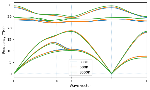
Command line phonon monitoring

This simple command line interface to the phonon plotting function allows for quick monitoring of the phonon calculation. If the sixelplot package is installed it is even possible to plot hi-res plots in the remote terminal supporting sixel standard (e.g. mlterm, xterm on Linux, iterm2 on OSX).

$ plot-bands --help

Usage: plot-bands [OPTIONS] [BANDS]...

  Plot the phonon dispersion from the file generated by ALAMODE. Optionally
  write out the plot to the output graphics file.

Options:
  -s, --sixel         Use SixEl driver for terminal graphics.
  -n, --nodecor       Decorate the plot.
  -w, --width FLOAT   Width of the figure.
  -h, --height FLOAT  Height of the figure.
  -o, --output PATH   Write output to the file.
  -l, --label TEXT    Label(s) for the plot. Comma-separated list
  -x                  Make plot in an interactive window
  -V, --version       Show the version and exit.
  --help              Show this message and exit.

$ plot-bands -w 7 -h 4 -l '300K,600K,3000K' example/VASP_3C-SiC_calculated/2x2x2/T_300K/phon/cryst.bands example/VASP_3C-SiC_calculated/2x2x2/T_600K/phon/cryst.bands example/VASP_3C-SiC_calculated/2x2x2/T_3000K/phon/cryst.bands